How to generate an LDA Topic Model for Text Analysis
In natural language processing, latent Dirichlet allocation (LDA) is a “generative statistical model” that allows sets of observations to be explained by unobserved groups that explain why some parts of the data are similar. So this is categorized as unsupervised learning. For example, if observations are words collected into documents, it posits that each document is a mixture of a small number of topics and that each word’s presence is attributable to one of the document’s topics. LDA is an example of a topic model.
I am going to use python’s the most popular machine learning library — Scikit learn.
0. Introduction
In this tutorial, we’ll use the reviews in the following dataset to generate topics from the reviews. In this way, we can know about what users are talking about, what they are focusing on, and perhaps where app developers should make progress at.
Data Source:
Google Play Store Apps Dataset : Web scraped data of 10,000 Play Store apps for analyzing the Android market.
1. Read Data
Import packages needed:
# Run in terminal or command prompt
# python3 -m spacy download enimport numpy as np
import pandas as pd
import re, nltk, spacy, gensim# Sklearn
from sklearn.decomposition import LatentDirichletAllocation, TruncatedSVD
from sklearn.feature_extraction.text import CountVectorizer, TfidfVectorizer
from sklearn.model_selection import GridSearchCV
from pprint import pprint# Plotting tools
import pyLDAvis
import pyLDAvis.sklearn
import matplotlib.pyplot as plt
%matplotlib inline
Read Data:
df = pd.read_csv(‘googleplaystore_user_reviews.csv’, error_bad_lines=False)
df = df.dropna(subset=[‘Translated_Review’])
2. Data Cleaning
# Convert to list
data = df.Translated_Review.values.tolist()# Remove Emails
data = [re.sub(r'\S*@\S*\s?', '', sent) for sent in data]# Remove new line characters
data = [re.sub(r'\s+', ' ', sent) for sent in data]# Remove distracting single quotes
data = [re.sub(r"\'", "", sent) for sent in data]pprint(data[:1])

3. Tokenize
Now we want to tokenize each sentence into a list of words, removing punctuations and unnecessary characters altogether.
Tokenization is the act of breaking up a sequence of strings into pieces such as words, keywords, phrases, symbols and other elements called tokens. Tokens can be individual words, phrases or even whole sentences. In the process of tokenization, some characters like punctuation marks are discarded.
We used Gensim here, use (deacc=True) to remove the punctuations.
def sent_to_words(sentences):
    for sentence in sentences:
        yield(gensim.utils.simple_preprocess(str(sentence), deacc=True))  # deacc=True removes punctuationsdata_words = list(sent_to_words(data))print(data_words[:1])

4. Stemming
Stemming is the process of reducing a word to its word stem that affixes to suffixes and prefixes or to the roots of words known as a lemma.
The advantage of this is, we get to reduce the total number of unique words in the dictionary. As a result, the number of columns in the document-word matrix (created by CountVectorizer in the next step) will be denser with lesser columns. You can expect better topics to be generated in the end.
def lemmatization(texts, allowed_postags=['NOUN', 'ADJ', 'VERB', 'ADV']): #'NOUN', 'ADJ', 'VERB', 'ADV'
    texts_out = []
    for sent in texts:
        doc = nlp(" ".join(sent))
        texts_out.append(" ".join([token.lemma_ if token.lemma_ not in ['-PRON-'] else '' for token in doc if token.pos_ in allowed_postags]))
    return texts_out
The Spacy package we used here is my favorite stemming package, I think is better than PorterStemmer, Snowball
# Initialize spacy ‘en’ model, keeping only tagger component (for efficiency)
# Run in terminal: python -m spacy download en
nlp = spacy.load(‘en’, disable=[‘parser’, ‘ner’])# Do lemmatization keeping only Noun, Adj, Verb, Adverb
data_lemmatized = lemmatization(data_words, allowed_postags=[‘NOUN’, ‘VERB’]) #select noun and verbprint(data_lemmatized[:2])

5. Create the Document-Word matrix
The LDA topic model algorithm requires a document word matrix as the main input.
You can create one using CountVectorizer. In the below code, I have configured the CountVectorizer to consider words that has occurred at least 10 times (min_df), remove built-in english stopwords, convert all words to lowercase, and a word can contain numbers and alphabets of at least length 3 in order to be qualified as a word.
vectorizer = CountVectorizer(analyzer='word',
                             min_df=10,
# minimum reqd occurences of a word
                             stop_words='english',
# remove stop words
                             lowercase=True,
# convert all words to lowercase
                             token_pattern='[a-zA-Z0-9]{3,}',
# num chars > 3
                             # max_features=50000,
# max number of uniq words    )data_vectorized = vectorizer.fit_transform(data_lemmatized)
6. Build LDA model with sklearn
Everything is ready to build a Latent Dirichlet Allocation (LDA) model. Let’s initialise one and call fit_transform() to build the LDA model.
For this example, I have set the n_topics as 20 based on prior knowledge about the dataset. Later we will find the optimal number using grid search.
# Build LDA Model
lda_model = LatentDirichletAllocation(n_components=20,               # Number of topics
                                      max_iter=10,
# Max learning iterations
                                      learning_method='online',
                                      random_state=100,
# Random state
                                      batch_size=128,
# n docs in each learning iter
                                      evaluate_every = -1,
# compute perplexity every n iters, default: Don't
                                      n_jobs = -1,
# Use all available CPUs
                                     )
lda_output = lda_model.fit_transform(data_vectorized)print(lda_model)  # Model attributes
Because we want to find out the best parametres, we use Latent Dirichlet Allocation with online variational Bayes algorithm:
LatentDirichletAllocation(batch_size=128, doc_topic_prior=None,
 evaluate_every=-1, learning_decay=0.7,
 learning_method=’online’, learning_offset=10.0,
 max_doc_update_iter=100, max_iter=10, mean_change_tol=0.001,
 n_components=10, n_jobs=-1, n_topics=20, perp_tol=0.1,
 random_state=100, topic_word_prior=None,
 total_samples=1000000.0, verbose=0)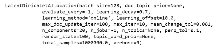
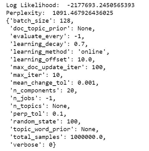
7. Diagnose model performance with perplexity and log-likelihood
A model with higher log-likelihood and lower perplexity (exp(-1. * log-likelihood per word)) is considered to be good.
# Log Likelyhood: Higher the better
print("Log Likelihood: ", lda_model.score(data_vectorized))# Perplexity: Lower the better. Perplexity = exp(-1. * log-likelihood per word)
print("Perplexity: ", lda_model.perplexity(data_vectorized))# See model parameters
pprint(lda_model.get_params())
On a different note, perplexity might not be the best measure to evaluate topic models because it doesn’t consider the context and semantic associations between words.
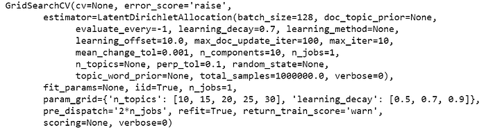
8. Use GridSearch to determine the best LDA model.
The most important tuning parameter for LDA models is n_components (number of topics).
In addition, I am going to search learning_decay (which controls the learning rate) as well.
Besides these, other possible search params could be learning_offset (downweigh early iterations. Should be > 1) and max_iter. These could be worth experimenting if you have enough computing resources. Be warned, the grid search constructs multiple LDA models for all possible combinations of param values in the param_grid dict. So, this process can consume a lot of time and resources.
# Define Search Param
search_params = {'n_components': [10, 15, 20, 25, 30], 'learning_decay': [.5, .7, .9]}# Init the Model
lda = LatentDirichletAllocation(max_iter=5, learning_method='online', learning_offset=50.,random_state=0)# Init Grid Search Class
model = GridSearchCV(lda, param_grid=search_params)# Do the Grid Search
model.fit(data_vectorized)GridSearchCV(cv=None, error_score='raise',
       estimator=LatentDirichletAllocation(batch_size=128, doc_topic_prior=None,
             evaluate_every=-1, learning_decay=0.7, learning_method=None,
             learning_offset=10.0, max_doc_update_iter=100, max_iter=10,
             mean_change_tol=0.001, n_components=10, n_jobs=1,
             n_topics=None, perp_tol=0.1, random_state=None,
             topic_word_prior=None, total_samples=1000000.0, verbose=0),
       fit_params=None, iid=True, n_jobs=1,
       param_grid={'n_topics': [10, 15, 20, 25, 30], 'learning_decay': [0.5, 0.7, 0.9]},
       pre_dispatch='2*n_jobs', refit=True, return_train_score='warn',
       scoring=None, verbose=0)
# Best Model
best_lda_model = model.best_estimator_# Model Parameters
print("Best Model's Params: ", model.best_params_)# Log Likelihood Score
print("Best Log Likelihood Score: ", model.best_score_)# Perplexity
print("Model Perplexity: ", best_lda_model.perplexity(data_vectorized))

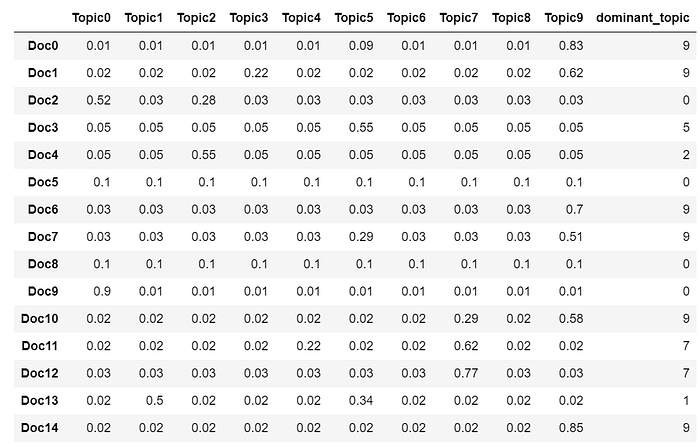
9. Dominant topic
To classify a document as belonging to a particular topic, a logical approach is to see which topic has the highest contribution to that document and assign it. In the table below, I’ve greened out all major topics in a document and assigned the most dominant topic in its own column.
# Create Document — Topic Matrix
lda_output = best_lda_model.transform(data_vectorized)# column names
topicnames = [“Topic” + str(i) for i in range(best_lda_model.n_components)]# index names
docnames = [“Doc” + str(i) for i in range(len(data))]# Make the pandas dataframe
df_document_topic = pd.DataFrame(np.round(lda_output, 2), columns=topicnames, index=docnames)# Get dominant topic for each document
dominant_topic = np.argmax(df_document_topic.values, axis=1)
df_document_topic[‘dominant_topic’] = dominant_topic# Styling
def color_green(val):
 color = ‘green’ if val > .1 else ‘black’
 return ‘color: {col}’.format(col=color)def make_bold(val):
 weight = 700 if val > .1 else 400
 return ‘font-weight: {weight}’.format(weight=weight)# Apply Style
df_document_topics = df_document_topic.head(15).style.applymap(color_green).applymap(make_bold)
df_document_topics
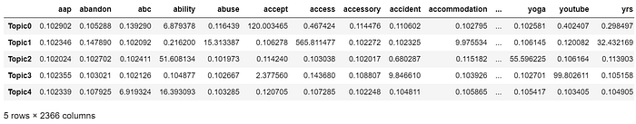
# Topic-Keyword Matrix
df_topic_keywords = pd.DataFrame(best_lda_model.components_)# Assign Column and Index
df_topic_keywords.columns = vectorizer.get_feature_names()
df_topic_keywords.index = topicnames# View
df_topic_keywords.head()
Get the top 15 keywords each topic:
# Show top n keywords for each topic
def show_topics(vectorizer=vectorizer, lda_model=lda_model, n_words=20):
    keywords = np.array(vectorizer.get_feature_names())
    topic_keywords = []
    for topic_weights in lda_model.components_:
        top_keyword_locs = (-topic_weights).argsort()[:n_words]
        topic_keywords.append(keywords.take(top_keyword_locs))
    return topic_keywordstopic_keywords = show_topics(vectorizer=vectorizer, lda_model=best_lda_model, n_words=15)# Topic - Keywords Dataframe
df_topic_keywords = pd.DataFrame(topic_keywords)
df_topic_keywords.columns = ['Word '+str(i) for i in range(df_topic_keywords.shape[1])]
df_topic_keywords.index = ['Topic '+str(i) for i in range(df_topic_keywords.shape[0])]
df_topic_keywords

At this step, we need to infer topics according to their key words. For example: For topic 3, people talk about “card”, “video” “spend”, we conclude that this topic is about “Card Payment”.
Next, put the 10 topics we infered into the dataframe.
Topics = ["Update Version/Fix Crash Problem","Download/Internet Access","Learn and Share","Card Payment","Notification/Support",
          "Account Problem", "Device/Design/Password", "Language/Recommend/Screen Size", "Graphic/ Game Design/ Level and Coin", "Photo/Search"]
df_topic_keywords["Topics"]=Topics
df_topic_keywords
10. Predict Topics using LDA model
Assuming that you have already built the topic model, you need to take the text through the same routine of transformations and before predicting the topic.
For our case, the order of transformations is:
sent_to_words() –> Stemming() –> vectorizer.transform() –> best_lda_model.transform()
You need to apply these transformations in the same order. So to simplify it, let’s combine these steps into a predict_topic() function.
# Define function to predict topic for a given text document.
nlp = spacy.load('en', disable=['parser', 'ner'])def predict_topic(text, nlp=nlp):
    global sent_to_words
    global lemmatization# Step 1: Clean with simple_preprocess
    mytext_2 = list(sent_to_words(text))# Step 2: Lemmatize
    mytext_3 = lemmatization(mytext_2, allowed_postags=['NOUN', 'ADJ', 'VERB', 'ADV'])# Step 3: Vectorize transform
    mytext_4 = vectorizer.transform(mytext_3)# Step 4: LDA Transform
    topic_probability_scores = best_lda_model.transform(mytext_4)
    topic = df_topic_keywords.iloc[np.argmax(topic_probability_scores), 1:14].values.tolist()

    # Step 5: Infer Topic
    infer_topic = df_topic_keywords.iloc[np.argmax(topic_probability_scores), -1]

    #topic_guess = df_topic_keywords.iloc[np.argmax(topic_probability_scores), Topics]
    return infer_topic, topic, topic_probability_scores# Predict the topic
mytext = ["Very Useful in diabetes age 30. I need control sugar. thanks Good deal"]
infer_topic, topic, prob_scores = predict_topic(text = mytext)
print(topic)
print(infer_topic)

Predict topics of our reviews in the original dataset:
def apply_predict_topic(text):
 text = [text]
 infer_topic, topic, prob_scores = predict_topic(text = text)
 return(infer_topic)df["Topic_key_word"]= df['Translated_Review'].apply(apply_predict_topic)
df.head()

Let’s take a look at the distribution of the prediction result.
df.groupby(‘Topic_key_word’).nunique()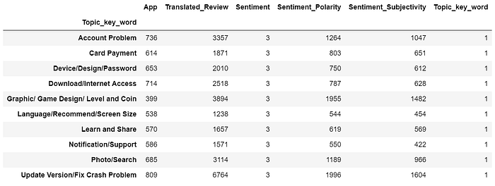
Output prediction result:
df.to_csv(“googlePlayStore_review_LDA.csv”)11. How to cluster documents that share similar topics and plot?
You can use k-means clustering on the document-topic probabilioty matrix, which is nothing but lda_output object. Since out best model has 15 clusters, I’ve set n_clusters=15 in KMeans().
Alternately, you could avoid k-means and instead, assign the cluster as the topic column number with the highest probability score.
We now have the cluster number. But we also need the X and Y columns to draw the plot.
For the X and Y, you can use SVD on the lda_output object with n_components as 2. SVD ensures that these two columns captures the maximum possible amount of information from lda_output in the first 2 components.
# Construct the k-means clusters
from sklearn.cluster import KMeans
clusters = KMeans(n_clusters=15, random_state=100).fit_predict(lda_output)# Build the Singular Value Decomposition(SVD) model
svd_model = TruncatedSVD(n_components=2)  # 2 components
lda_output_svd = svd_model.fit_transform(lda_output)# X and Y axes of the plot using SVD decomposition
x = lda_output_svd[:, 0]
y = lda_output_svd[:, 1]# Weights for the 15 columns of lda_output, for each component
print("Component's weights: \n", np.round(svd_model.components_, 2))# Percentage of total information in 'lda_output' explained by the two components
print("Perc of Variance Explained: \n", np.round(svd_model.explained_variance_ratio_, 2))

We have the X, Y and the cluster number for each document.
Let’s plot the document along the two SVD decomposed components. The color of points represents the cluster number (in this case) or topic number.
# Plot
plt.figure(figsize=(12, 12))
plt.scatter(x, y, c=clusters)
plt.xlabel('Component 2')
plt.xlabel('Component 1')
plt.title("Segregation of Topic Clusters", )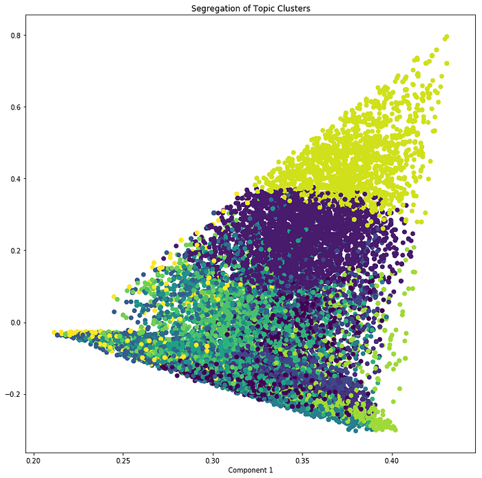
12. Get similar documents for any given piece of text?
Once you know the probaility of topics for a given document (using predict_topic()), compute the euclidean distance with the probability scores of all other documents.
The most similar documents are the ones with the smallest distance.
from sklearn.metrics.pairwise import euclidean_distancesnlp = spacy.load('en', disable=['parser', 'ner'])def similar_documents(text, doc_topic_probs, documents = data, nlp=nlp, top_n=5, verbose=False):
    topic, x  = predict_topic(text)
    dists = euclidean_distances(x.reshape(1, -1), doc_topic_probs)[0]
    doc_ids = np.argsort(dists)[:top_n]
    if verbose:
        print("Topic KeyWords: ", topic)
        print("Topic Prob Scores of text: ", np.round(x, 1))
        print("Most Similar Doc's Probs:  ", np.round(doc_topic_probs[doc_ids], 1))
    return doc_ids, np.take(documents, doc_ids)
Get similar documents:
mytext = [“I think they are really helpful”]
doc_ids, docs = similar_documents(text=mytext, doc_topic_probs=lda_output, documents = data, top_n=1, verbose=True)
print(‘\n’, docs[0][:500])
print()